Copyright © Thomas Fetter
2014-2026

After developing the Mathcad model of the dynamics of a rocket's flight, I started to look for a way to do a better job of visualizing the attitude of the rocket during the flight. Mathcad works nicely for solving equations numerically and creating static plots, but it cannot create a realtime rendering of the rocket showing its attitude, or angular position in space. Having such a realtime visualization can help to gain insight into the dynamics of the rocket's flight.
Since Mathcad cannot do this, I used the popular, easy to use (and free) programming language, Python. Python is an open source language, so it has many has many extensions. I use the VPython extension that adds high level commands for 3-D rendering. I then take the numerical output from Mathcad that describes the rockets flight trajectory, and then animate a 3-D model in VPython. To see a video of a flight visualization, see the table on the Flight Data Analysis page. Python does not need to be installed on your computer to see the videos.
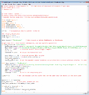
The VPython visualization code is broken into three files. The main file, or module, is Rocket Dynamics Visualization 3D.py. This code reads the data files, creates the various graphing windows, does all the math for the visualizations, and then plots the graphs and draws the visualizations.
The rocketobjects.py module creates all the 3D rocket objects (nosecone, body tube, fins, and rocket) as classes that are used by the main program to render the orientation visualizations. Once the object rocket instance is created, the main program only needs to update the location and orientation of the object.
The rocketequations.py module contains the math functions that are used by the main program module to do the axis translation.
Here are the VPython files:
Rocket Dynamics Visualization 3D.py
rocketobjects.py
rocketequations.py
Note: t\his code must be run from the VIDLE user interface that is a part of the VPython installation.
I use the Python programming language for doing the realtime visualization. Python is a widely used open source language, its available for free download, and it has many has many extension libraries. I use the graphics capability of VPython, a graphical programming extension module for Python, to do the 3D rendering, and PyWin, which provides a Windows interface.
To install Python on your computer to access and run the visualization program:
First install Python 2.7
Then install pywin
Then install Vpython
Note, VPython automatically installs the NumPy library.
The visualization code was written using Python 2.7. I used the "new style" for the rocketobjects classes, and the rest of the code is non-specific, so this code should run under Python 3.3. I will be upgrading to Python 3.3 shortly, and will verify compatibility.
If rocketobjects.py and rocketequations.py are installed in the same directory as Rocket Dynamics Visualization 3D.py, Python will find the necessary modules automatically.
Line 44 in the Rocket Dynamics Visualization 3D.py file must be modified to point to the location of the data flight simulation spreadsheet on your computer.
I will be providing more detailed documentation for the Python code in the future.
By adapting the Python program I wrote to visualize the results of my 3D flight simulator, and using the data from the RAF Data Logger, I am able to visualize the flight of an actual rocket. I take the data from the Data Logger, as well as data from a barometric altimeter and a GPS logger, and save these data into simple Excel spreadsheets. The Python visualization program then reads the data from the spreadsheets, performs the calculations needed to create the various graphs and plots, and then plots the data and draws the graphics, just as it does with the Mathcad flight simulation data.
The Data Logger provides 3-axis angular rotation rate data and 3-axis acceleration data. The Barrometric altimeter provides the altitude data. And the GPS provides the north-south/east-west location data. The z-axis velocith is calculated by integrating the acceleration data.
For the actual flight data, Lines 27 and 28 in the Rocket Dynamics Visualization 3D.py file must be modified to point to the location of these three spreadsheets on your computer. The samples rates must also be set for each data set depending on the particular altimeter and GPS unit used.
For visualizing the Mathcad flight simulation model, I take the output data from the Mathcad model that describes the rockets flight, including its orientation and position in space, and save these into simple Excel spreadsheets. The Python visualization program then reads the data from the spreadsheets, performs the calculations needed to create the various graphs and plots, and then plots the data and draws the graphics.
The rocket orientation is calculated using angular rate of change data from the rocket frame-of-reference. Although the Mathcad model also calculates the orientation of the rocket in the ground frame-of-reference, I do this calculation in the Python visualization program as this is necessary when the source of data for the visualization is actual flight data from a rate gyroscope (see below). By using the rocket frame rate of rotation data from the simulation, the Python visualization program processes the input date the same whether the source of the data is the simulation or actual flight data.
Brief Description of the Python Visualization Program
To get the absolute angular orientation in the fixed ground frame-of-reference, the axes must be translated from the rocket frame-of-reference to the ground frame-of-reference. There are a number of different axis translation methods; I use Euler's angles. Euler's angles are first calculated using the instantaneous angular rate-of-change for each of the three rocket axes, and then a ground frame-of-reference orientation vector is calculated from the Euler angles.
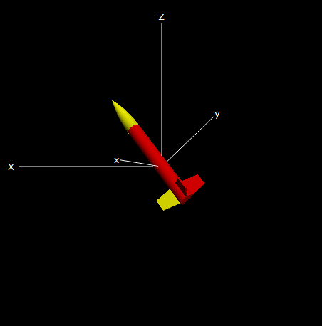
The rocket's angular orientation is then drawn using a 3D representation of the rocket from two perspectives, a side view and a tops-down view. The tops-down view leaves a trail from the tip of the nosecone. If the rocket spins, the cross-coupling between the axes causes a small nutation, or looping motion of the rocket, that can be seen in the trail as it traces the path of the tip of the nosecone.
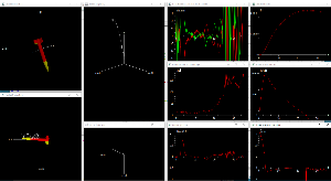
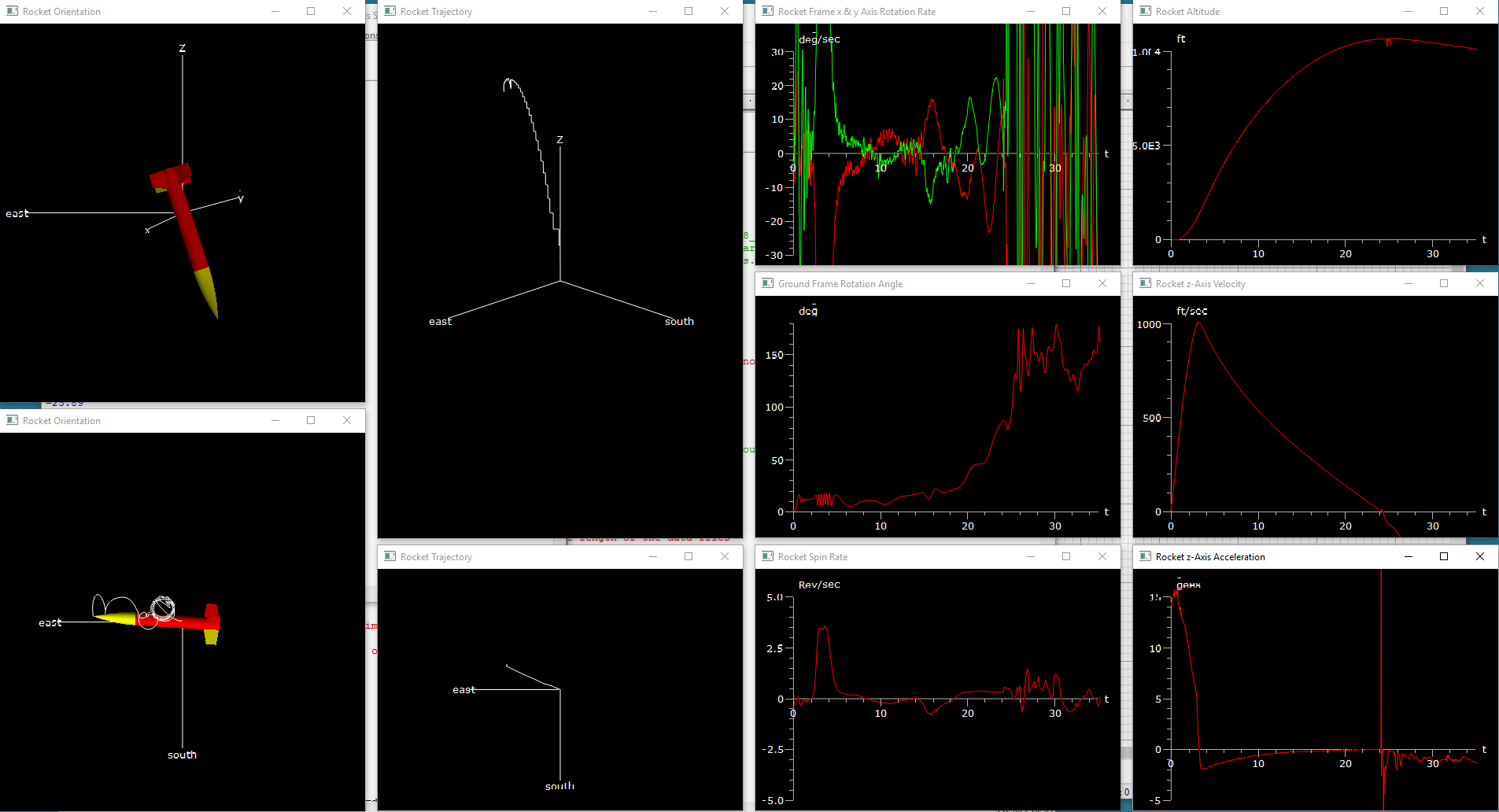
The picture on the left shows the visualizations and graphs rendered by the Python program (click the picture to enlarge).
The first two windows on the left are the rocket attitude renderings from a side view and top down view. The X-Y-Z axes are the ground frame of reference, and the x-y-z axes are the rocket frame of reference.
The next two windows show the location of the rocket in ground referenced 3-d space.
The next graph shows the rocket frame rotation rate about the x and y rocket frame axes (see the angular position rendering for the location of the x and y axes.
Below that is a graph of the angle of the rocket retaliative to the Z ground frame axis (ground frame up), or tilt.
The bottom graph shows the rotation rate of the rocket about it's z-axis (longitudinal axis).
The final column of graphs on the right side shows the altitude, the rocket z-axis velocity, and the rocket z-axis acceleration.
All the plots advance together in realtime.
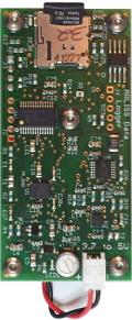
With the addition of data from a rate gyroscope, the same Python flight visualization program used to visualize the flight simulator data could be used to visualize the flight of actual rockets. Because there were no reasonably priced gyroscope sensors adapted to rocket use, I started a project to adapt Arduino based electronics to accomplish this. But, at the end of 2014, RAF Research introduced a Data Logger board that records 3-axis acceleration and rotational rates to onboard memory. It is designed for rocket use, so it has the necessary triggering to detect launch and record the flight. This is exactly what I was looking for!
The RAF AL-016 High Speed Data Logger was originally designed to investigate the forces being seen by the payloads on ARLISS flights. The Data Logger has a three-axis rate gyro and two three-axis accelerometers that are recorded to onboard memory. The Data Logger has an automatic launch detect sequence that initiates the recording of the data. The data can then be analyzed a by post-processing software application available from RAF Research that is focused analyzing the forces payload during the various phases of the flight including payload ejection.
Bob Feretich wrote a two part article that appears in the November/December 2015 and January/February 2016 issues of Spot Rocketry Magazine that describes the Arliss Data Logger Project.
At the end of 2014, I purchased an RAF AL-016 High Speed Data Logger board. I planned to fly the Data Logger at the Tripoli Central Dairy Aire launch in May of 2015, that launch was canceled due to rain, so my first flights of the Data Logger were at Tripoli Central's October Skies launch in October 2015.
What is nice about the RAF Data Logger is it is designed for high power rocketry use. I flew it twice at October Skies, and both times, it worked flawlessly, and I got good data from both flights.
Click here to see flight visualizations using the data from the RAF Data Logger.
RAF Research AL-016 High Speed Data Logger
Photo courtesy of RAF Reasearch